Processing Large Datasets with Xarray, Dask, and Zarr

In the era of big data analytics, scientists and data engineers often face the challenge of processing datasets that are too large to fit into memory. This is particularly common in climate science, remote sensing, and other fields dealing with large multidimensional arrays. I’ll show you that with a combination of Xarray, Dask, and Zarr, working with massive datasets is not just possible, but efficient and intuitive.

Why Xarray, Dask, and Zarr?

Xarray provides a convenient data model for labeled multi-dimensional arrays, similar to NetCDF. Dask offers out-of-core computing and parallel processing of chunked datasets. Zarr is an efficient, chunked, binary storage format that integrates seamlessly with Xarray and Dask, allowing partial I/O and parallel writes.

Key benefits include:

• Lazy evaluation: Computations are only carried out when you explicitly request them to compute, helping avoid loading unnecessary data into memory.
• Parallel processing: Dask can distribute computations across multiple threads or worker processes on one machine, or even an HPC cluster or cloud environment.
• Chunked storage and access: Zarr neatly stores large datasets in chunks, enabling efficient reading and writing of partial data.
• Intuitive labeling: Dimensions and coordinates are labeled, making data manipulation more transparent.
• Scalability: The same code can often scale from a single laptop to a multi-node cluster.

Quick Installation

pip install xarray dask zarr netCDF4 matplotlib kerchunk

Go ahead and install kerchunk as well, since it is increasingly useful for handling large ensembles of data in remote storage (e.g., cloud object storage).

Basic Setup

import xarray as xr
import dask.array as da
from dask.distributed import Client
import matplotlib.pyplot as plt

# Initialize a local Dask client
client = Client()
print(f"Dask dashboard available at: {client.dashboard_link}")

Opening a Zarr Dataset

Zarr is an excellent format for storing large multidimensional data. Suppose you have a climate dataset in Zarr format:

# Open a Zarr dataset with Xarray
ds = xr.open_zarr('path/to/climate_data.zarr')
print(f"Dataset dimensions: {ds.dims}")
print(f"Dataset variables: {list(ds.data_vars)}")

Tip: If your dataset is on cloud storage (e.g., S3), you can still open it with xr.open_zarr() by specifying a cloud-based path. Just ensure you have the appropriate credentials or public access.

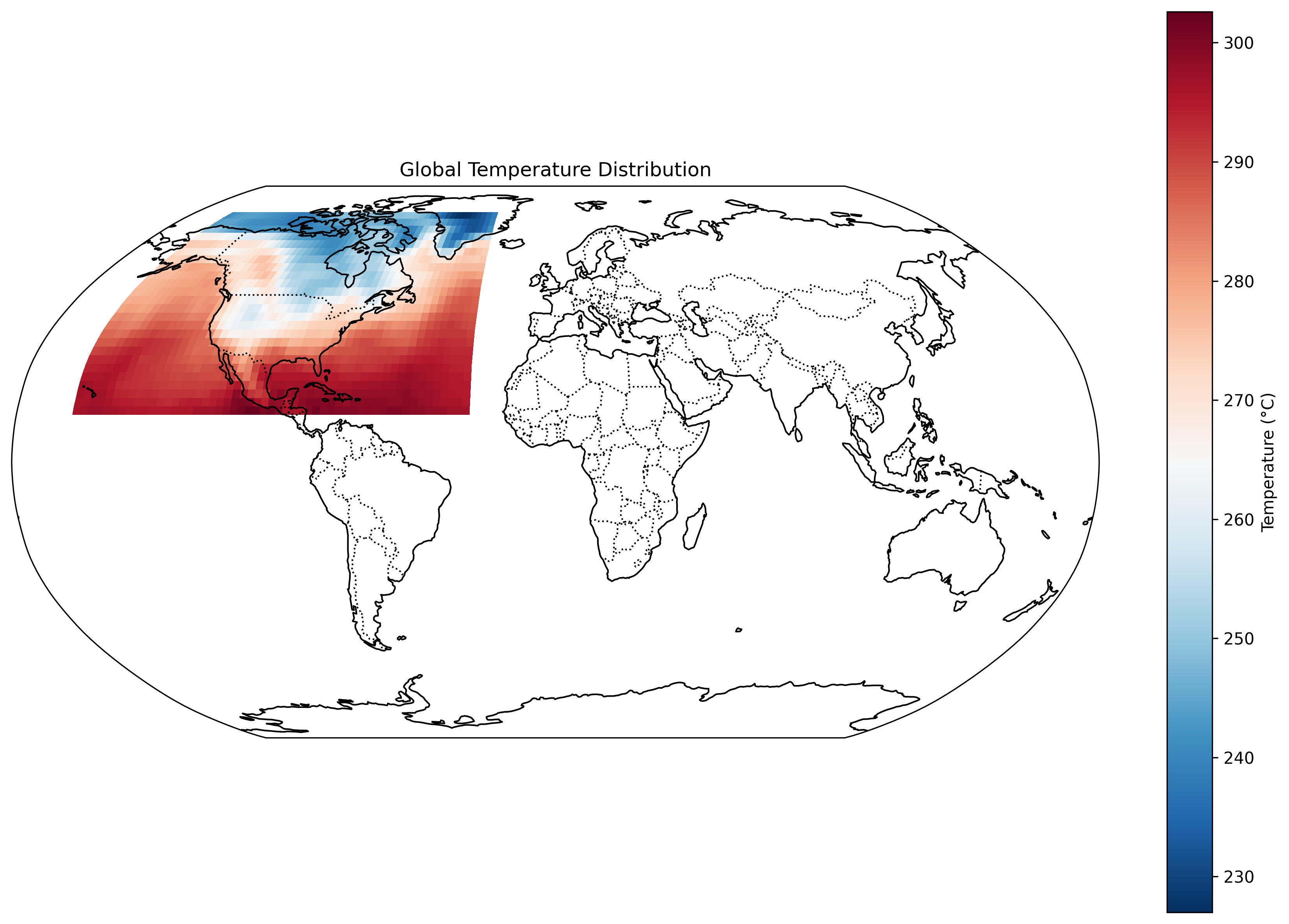
Lazy Computations and Anomaly Calculation

Dask works with Xarray so that operations are merely planned rather than executed immediately. For instance, let’s say we want to compute monthly temperature anomalies:

# Calculate the climatological mean (baseline)
climatology = ds['temperature'].groupby('time.month').mean('time')

# Calculate anomalies
anomalies = ds['temperature'].groupby('time.month') - climatology

# The computations above haven't happened yet (they are lazy operations)
print("Computation plan created, but not yet executed.")

We can continue chaining further operations without using up memory, since Dask composes a task graph. Here’s an example of temperature anomalies over time:

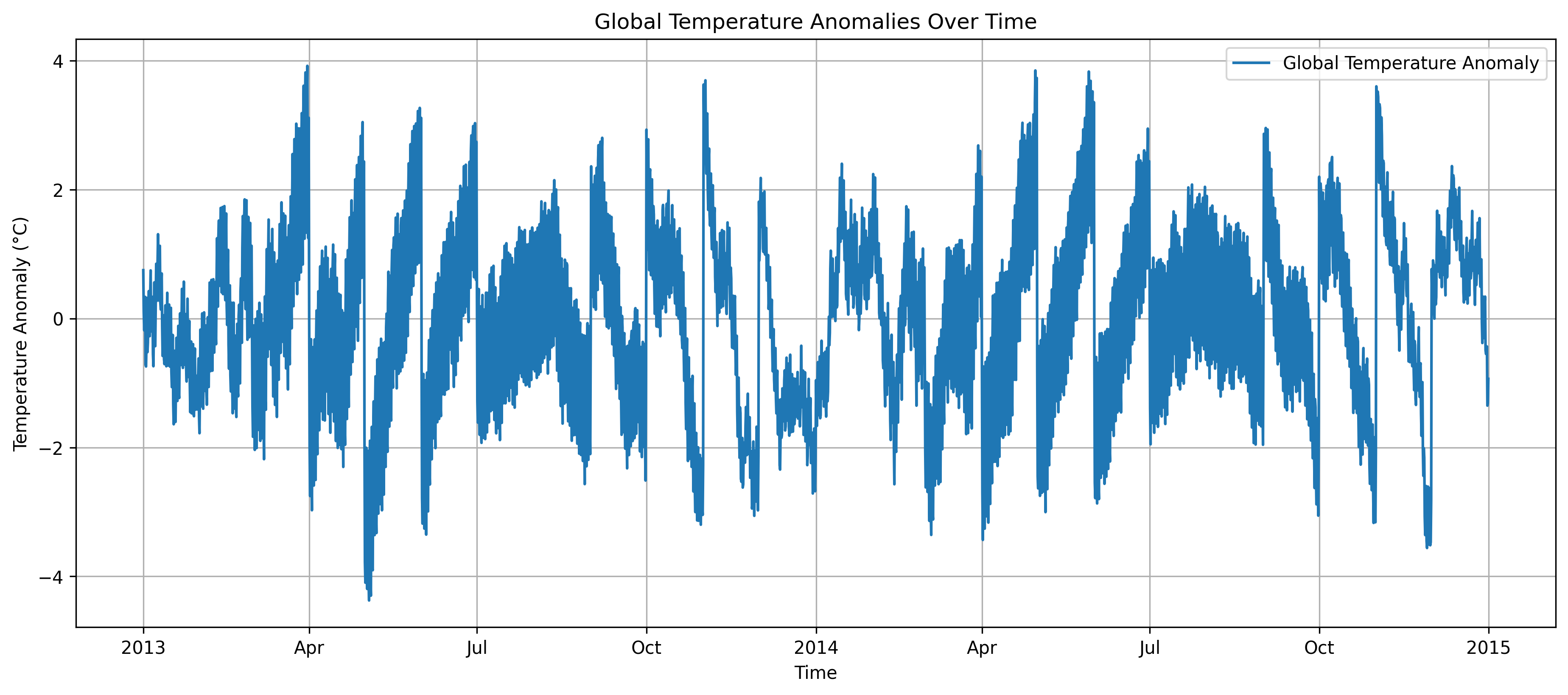
This plot shows how global mean temperature anomalies vary over time, computed efficiently using Dask’s lazy evaluation and parallel processing capabilities.

Understanding Data Chunking

One of the key concepts in working with large datasets is chunking. Here’s a visualization of how our data is chunked:

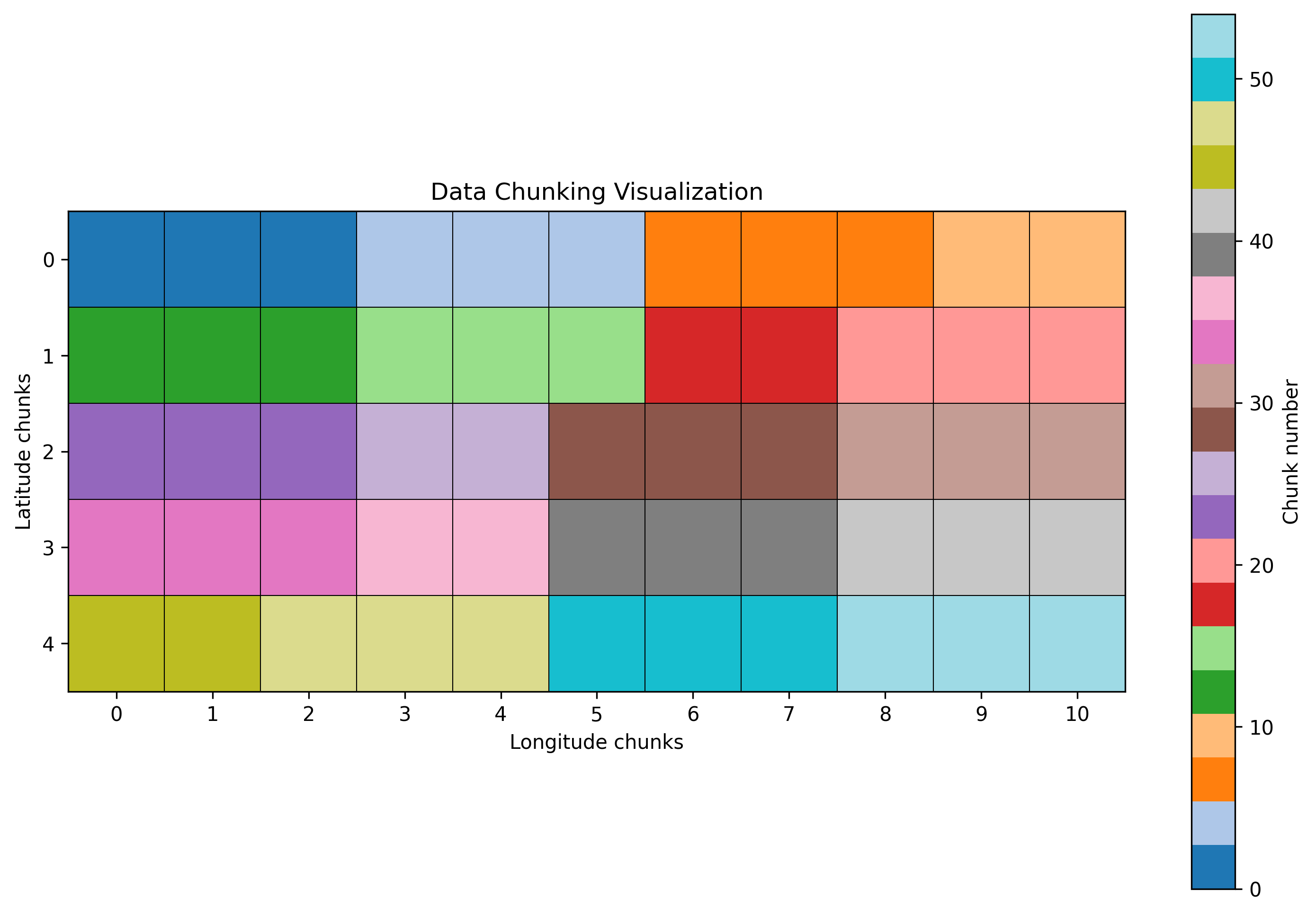
Each colored block represents a chunk of data that can be processed independently. This chunking strategy allows for:

• Parallel processing of different chunks
• Loading only the necessary portions of data
• Efficient storage and retrieval
• Optimal memory usage during computations

The choice of chunk size is crucial for performance. Too small chunks create overhead from many small computations, while too large chunks may not fit in memory.

Efficient Data Writing

One of Zarr’s key advantages is its ability to write data in parallel. Below, we chunk anomalies and store them as a new Zarr dataset:

# Define chunking for efficient parallel writes
chunk_sizes = {'time': 365, 'latitude': 50, 'longitude': 50}
anomalies.chunk(chunk_sizes).to_zarr('temperature_anomalies.zarr', mode='w')

Handling Large or Many Files in Parallel

Using Dask for Large-Scale Multi-File Processing

When dealing with a large set of files (e.g., daily NetCDF files spanning decades), you can leverage Dask’s parallel computing to process them efficiently:

ds_all = xr.open_mfdataset(
    "path/to/daily_files/*.nc",
    parallel=True,
    combine='by_coords',
    chunks={'time': 365, 'latitude': 50, 'longitude': 50}
)

• open_mfdataset: Allows you to open multiple files as if they were one large dataset.
• parallel=True: Splits file reads across multiple Dask workers.
• combine='by_coords': Ensures that variables and coordinates from different files are merged correctly.

You can then perform the same operations (like computing anomalies, means, etc.) on this combined dataset. Even though you might have hundreds of files, Dask will orchestrate the reading and processing efficiently, chunk by chunk.

Scaling to HPC and the Cloud

• For HPC clusters, you can run Dask on a job scheduler (like Slurm) and create a Dask cluster with one scheduler and multiple workers across nodes.
• In the cloud (AWS, GCP, Azure), you can create a Dask cluster on managed services or Kubernetes where each node is a Dask worker. Your code remains largely the same, but now can scale out seamlessly.

Kerchunk

Kerchunk provides a mechanism to describe and consolidate chunked data references (e.g., for many NetCDF or GRIB files in cloud object storage) into a single JSON reference file. This allows Xarray (in combination with FSSpec) to open remote data without needing to download or combine every file locally.

For example, if you have thousands of NetCDF files in a cloud bucket, Kerchunk can create a “virtual” single dataset by generating a reference JSON with information about each chunk’s location. You can then do:

import fsspec
import ujson
from kerchunk.hdf import SingleHdf5ToZarr

# Example: building a kerchunk reference for one large NetCDF file
url = "https://bucket-name/path/to/data.nc"
fs = fsspec.open(url)
m = SingleHdf5ToZarr(fs.open(url), url)
with open("reference.json", "w") as f:
    f.write(ujson.dumps(m.translate()))

# Now open the reference as if it's a Zarr store
ds_kerchunk = xr.open_dataset(
    fsspec.get_mapper("reference.json"),
    engine="zarr",
    chunks={}
)
print(ds_kerchunk)

This approach is especially useful when working with large stores of remote data. Rather than reading raw data from every file, you can read only from specific chunks as needed, accelerate queries, and reduce data transfers.

Performance Tips

1. Chunk Size Optimization

Choosing the right chunk size is critical for performance. Too small, and Dask overhead dominates; too large, and memory usage spikes:

ds = ds.chunk({'time': 'auto', 'latitude': 100, 'longitude': 100})

2. Control Parallel Workers

Ensure you have enough workers to process your tasks efficiently—but without oversubscribing the machine:

client = Client(n_workers=4, threads_per_worker=2)

3. Monitor Memory

Use the Dask dashboard to check memory usage and identify bottlenecks:

client.dashboard_link

Complete Example

Below is a short, end-to-end example showing how all these ideas fit together:

import xarray as xr
import dask.array as da
from dask.distributed import Client
import matplotlib.pyplot as plt

# 1. Initialize Dask
client = Client(n_workers=4)
print(f"Dashboard link: {client.dashboard_link}")

# 2. Open dataset (Zarr or use kerchunk references)
ds = xr.open_zarr('climate_data.zarr')

# 3. Rechunk for performance
ds = ds.chunk({'time': 365, 'latitude': 50, 'longitude': 50})

# 4. Calculate climatology and anomalies
climatology = ds['temperature'].groupby('time.month').mean('time')
anomalies = ds['temperature'].groupby('time.month') - climatology

# 5. Calculate global mean anomalies
global_mean = anomalies.mean(dim=['latitude', 'longitude'])

# 6. Compute results
result = global_mean.compute()

# 7. Visualize
plt.figure(figsize=(12, 6))
result.plot()
plt.title('Global Temperature Anomalies')
plt.show()

# 8. Save out results in Zarr
result.to_zarr('processed_results.zarr', mode='w')

Running on a single workstation or a multi-node cluster, you can handle datasets that would otherwise be impossible to open using traditional in-memory approaches.

Further Resources:

• Dask: https://www.dask.org/
• Xarray: https://docs.xarray.dev/en/stable/
• Zarr: https://zarr.readthedocs.io/en/stable/
• Kerchunk: https://github.com/fsspec/kerchunk