MongoDB + Uber H3 = Fast global datasets
As a researcher grappling with environmental datasets, the slow speed of database queries can often hinder your progress and disrupt the process of problem-solving. This article presents a robust solution to accelerate geospatial database queries, employing an optimized database structure fortified by Uber’s H3 index. This discussion will encompass an explanation of how Uber’s H3 index functions, supplemented by a coding example to facilitate further implementation.
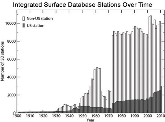
Before delving into the solution, it is imperative to understand the core issue. For instance, consider the ISD (Integrated Surface Database) by NOAA, comprising approximately 2.6 billion single weather measurements spanning from 1901 to the present. Our objective is to insert this data into a database for rapid querying, enabling its utilization in further applications. MongoDB once proposed a technique for this, which required substantial hardware resources. In this article, we combine MongoDB’s approach with Uber’s H3 index to achieve faster query execution.
The document displayed below is a MongoDB document in JSON format, encompassing a weather station ID (st), a timestamp (st), a geoJSON encoded location object, and the actual data.
{
  "st" : "u725053",
  "ts" : ISODate("2013-06-03T22:51:00Z"),
  "position" : {
    "type" : "Point",
    "coordinates" : [
        -96.4,
        39.117
    ]
  },
  "elevation" : 231,
  "airTemperature" : {
      "value" : 21.1,
      "quality" : "1"
  },
  "sky condition" : {
    "cavok": "N",
    "ceilingHeight": {
        "determination": "9",
        "quality": "1",
        "value": 1433
    }
  }
  "atmosphericPressure" : {
      "value" : 1009.7,
      "quality" : "5"
  }
  [etc]
}
As demonstrated by Avery from MongoDB’s blog, this query takes about 1500ms to execute using a configuration of 32 vCPUs, 251GB of RAM, 8 x 800GB SSD, and approximately 300ms with 100 instances of 16GB RAM machines.
db.data.find({"st" :db.data.find({"st" : "u103840",
              "ts" : {"$gte": ISODate("1989-01-01"),
              "$lt" : ISODate("1990-01-01")}})
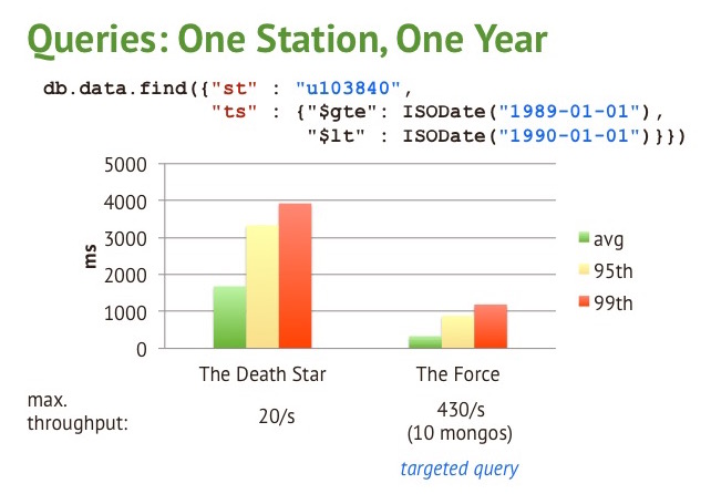 Left: Single machine (32 cores, etc.), Right: 100 smaller machines clustered | Image from https://www.mongodb.com/blog/post/weather-century-part-4
Although throwing more hardware at the problem might seem a feasible solution, the crux of the matter lies in the unoptimized database structure. Since all documents are housed in a single database, every data piece must be verified during query execution. In a production environment, it’s more commonplace to query by location rather than station ID, therefore our optimization will focus on location.
Introducing Uber’s H3 Index
This leads us to Uber’s H3 index. Uber’s open-sourced hexagonal hierarchical geospatial indexing system is proficient in segmenting the Earth into uniformly distributed hexagons across 16 resolution levels, making it a potent tool for a variety of applications.
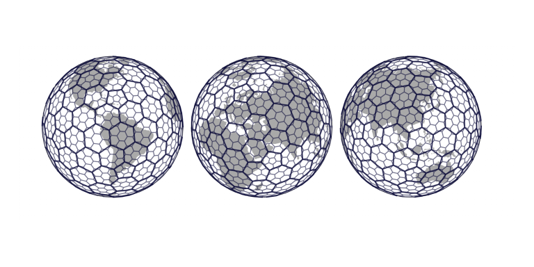
Bigger hexagon: lower resolution | Smaller hexagon: higher resolution https://eng.uber.com/h3/ Every hexagon is represented by a unique 16-bit hexadecimal index e.g.
8843a13687fffff
The resolution can be adapted based on the problem at hand. Each resolution level comprises a specific number of hexagons enveloping the entire globe, ranging from 122 hexagons at resolution 0 to over 500 trillion at resolution 15.
| H3 resolution | Average hexagon area | Average hexagon edge length | Number of hexagons |
|---|---|---|---|
| 0 | 4.25e+09 km² | 1.11e+06 km | 122 |
| 1 | 6.07e+08 km² | 3.78e+05 km | 842 |
| 2 | 8.67e+07 km² | 1.89e+05 km | 5882 |
| 3 | 1.24e+07 km² | 9.44e+04 km | 41176 |
| 4 | 1.77e+06 km² | 4.72e+04 km | 288122 |
| 5 | 2.53e+05 km² | 2.36e+04 km | 2016842 |
| 6 | 3.61e+04 km² | 1.18e+04 km | 14117894 |
| 7 | 5.16e+03 km² | 5.89e+03 km | 98825158 |
| 8 | 7.36e+02 km² | 2.95e+03 km | 691776106 |
| 9 | 1.05e+02 km² | 1.48e+03 km | 4842432742 |
| 10 | 1.50e+01 km² | 7.42e+02 km | 33897029194 |
| 11 | 2.14 km² | 3.71e+02 km | 237279204358 |
| 12 | 3.06e-01 km² | 1.86e+02 km | 1660954420506 |
| 13 | 4.37e-02 km² | 9.31e+01 km | 11626680943542 |
| 14 | 6.24e-03 km² | 4.66e+01 km | 81386766504794 |
| 15 | 8.91e-04 km² | 2.33e+01 km | 569707365533558 |
| https://h3geo.org/docs/core-library/restable/ |
Uber offers a C library for swift and convenient conversions from coordinates to the H3 index and vice versa. Additionally, bindings are available for all major languages.
Optimizing the Database Structure
Having established the foundational components, we can now design our database structure with two significant modifications:
- Each year will have a dedicated database
- Each year will incorporate 5882 tables of H3 indexes at resolution 2

This division allows us to distribute the Earth into 5882 uniform hexagons, drastically reducing the number of documents to be searched for each query, usually by a factor of 5882. A hexagon at resolution 2 possesses the following dimensions:
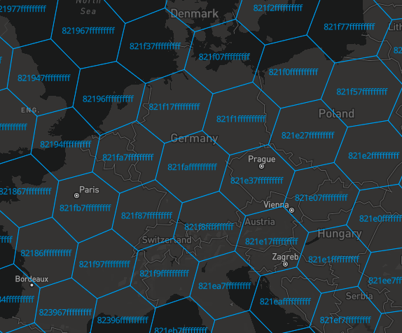
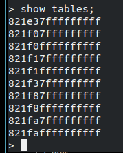
After inserting some data for Germany, the h3 index tables looks like:
This methodology is highly scalable, facilitated by a higher H3 resolution and distributed machines. Additionally, smaller areas with denser data (as per our approach at Predly) can be queried efficiently with this method.
Given the following query:
{
 "location" :{
            $near: {
                   $geometry: {
                               type: "Point" ,
                               coordinates: [ 8.25,50 ]
                              },
                               $maxDistance:1000,
                               $minDistance:10
                              }
                     }
 },
 "ts" : ISODate("1989-01-01")
}
The proposed workflow is as follows:
- Determine the years to query (in this case, 1989)
- Identify the desired H3 index: h3.geo_to_h3(50,8.25,2) = ‘821faffffffffff’
- Execute the query for the given database and table
An example would be like
def make_query(query):

    # get year
    if isinstance(query["ts"], datetime.date):
        ts = query["ts"]
        year = ts.year

    # get h3 index
    lon, lat = query["location"]["coordinates"]
    h3_index = h3.geo_to_h3(lat,lon,2)

    return db[year][h3_index].find(query)
In a global best-case scenario, this approach can accelerate query speed nearly 5882 times. It is hoped that this article piques your interest, and you find its insights valuable for your next big geospatial data project.